Table of Contents
Normality and Data transformation
Introduction
Data transformation is a powerful tool when the data don't look like forming a normal distribution. The idea of data transformation is that you convert your data so that you can assume the normality and use parametric tests. To determine whether we need any data transformation, we need to check the normality of the data. Although there are several statistical methods for checking the normality, what you should do is to look at a histogram and QQ-plot, and then run a test for checking the normality. You also should read the section for the differences of the two statistical methods explained in this page.
One important point of data transformation is that you must defend that your data transformation is legitimate. You cannot do arbitrary data transformation so that you can get results you want to get. Make sure you clarify why you do data transformation and why it is appropriate.
Histogram
We prepare data by using a random function. To be able to reproduce the results quickly, we set the seed for the random functions.
This means that we are randomly taking 20 samples from the normal distribution with mean = 0 and sd = 1. I set the specific seed so that you can reproduce the same data_normal. So, the values will be changed every time you execute this. In my case, it looked like this.
We will also prepare another kind of data for comparison.
data_exp are created from a different distribution (an exponential distribution).
One good practice before doing any statistical test for normality and data transformation is to look at the histogram of the data. This gives you a good picture of what the data look like, and whether you really need data transformation. In R, you can use hist() function to create a histogram.
The hist() function automatically selects the width of each bin in a histogram. You can try different algorithms to determined the number of bins by specifying the breaks option. In my experience, “FD” works well for many cases. Here is the example of histograms. To make the comparison easier, we put the two histograms into one window.

Q-Q plot
Another way to visually investigate whether data forms the normal distribution is to draw a Q-Q plot. A Q-Q plot shows the mapping between the distribution of the data and the ideal distribution (the normal distribution in this case). Let's take a look at it.
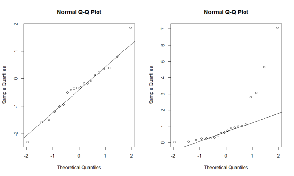
If your data are close to the normal distribution, most of the data points should be close to the line. So obviously, some of the data points in data_exp are far from the line, which means that it is less likely that data_exp were taken from the normal distribution.
Statistical tests for normality
If the histogram of your data doesn't really look like a normal distribution, you should try a statistical test to check the normality. Fortunately, this is pretty easy in R. There are two common tests you can use for the normality check.
Shapiro-Wilk test
One common test for checking the normality is Shapiro-Wilk test. This test works well even for a small sample size, so generally you just need to use this.
The null hypothesis of Shapiro-Wilk test is that the samples are taken from a normal distribution. So, if the p value is less than 0.05, you reject the hypothesis, and thinks that the samples are not taken from a normal distribution. In R, you just need to use shapiro.test() function to do Shapiro-Wilk test.
And you get the result.
In this case, you can still assume the normality. Let's try the same test with data_exp.
So, we reject the null hypothesis, and the samples are not considered to be taken from a normal distribution. Thus, you need to do data transformation or use a non-parametric test.
Kolmogorov-Smirnov test
Another test you can use for checking the normality is Kolmogorov-Smirnov test. This test basically checks whether two datasets are taken from the same distribution, but it can be used for comparing one dataset against an ideal distribution (int this case, a normal distribution). This test is also quite easy to do in R.
Here, we are comparing the data against a normal distribution (“pnorm”) with the mean and standard deviation calculated from the dataset.
The result says that we can still assume the normality. Let's take a look at the test with data_exp.
We reject the null hypothesis that data_exp were taken from the normal distribution.
Because Kolmogorov-Smirnov test is not only for comparing the dataset against the normal distribution, you can make a comparison with other kinds of distributions. Let's try to make a comparison between data_exp and an exponential distribution. You can use “pexp” instead of “pnorm”, but you need to be a little careful about calculating the mean and standard deviation for a log-normal transformation.
So, we can think that data_exp were more likely taken from a log-normal distribution rather a normal distribution. You can also use this test for comparing the two distributions (the null hypothesis is that both datasets were originated form the same distributions).
Which test should I use?
Generally, Kolmogorov-Smirnov test becomes less sensitive (less powerful to detect a significant effect) when the sample size is small. It is hard to say which number is considered as small or large, but it is said that Kolmogorov-Smirnov test is more appropriate if your sample size is the order of 1000.
However, some people use Kolmogorov-Smironov test even if they have a small sample size. One reason is probably that Shapiro-Wilk test is often too strict and often shows a significant result even if the true population has the normality. So it is fairly common that you see a significant result with Shapiro-Wilk test, but cannot see any significant result with Kolmogorov-Smirnov test.
A general practice on the normality tests I found is to run both tests and see the results. If both of the tests say that you cannot assume the normality, you may have to do a data transformation (explained later) or use a non-parametric test. Some of the parametric tests are fairly robust against the non-normality (particularly a t test and one-way ANOVA). The normality tests mentioned above need a large sample size (which may not be possible in HCI research). Thus, we don't need to be too strict to follow the results of the normality test. Furthermore, when the sample size is small, both tests usually are less powerful than what they should be. So blindly believing the results of those tests could be dangerous. Recently I found that a D'Agostino-Pearson omnibus test and Anderson–Darling test can work better for a small sample size, so please try to find information about these tests if you want to know more about normality tests.
Again, I suggest using a histogram and Q-Q plot. Even if they are subjective ways to check the normality, they still give you a good idea of whether your data really look like a normal distribution or not. So use these plots as well as statistical tests, and see whether you really need to do any data transformation or non-parametric test.
In conclusion, there is no perfect way to judge the normality of data. But histograms, Q-Q plots and normality tests are useful tools to see at least whether your data are really far from the normal distribution or not.
Data transformation
Once you decide to do data transformation, you need to pick up which transformation to use. Although you can do any kind of transformation, there are a few of transformation which are commonly used. You could do other kinds of transformation, but regardless of transformation, you must defend why you decided to use that transformation and why it is appropriate.
You can do parametric tests after you do data transformation. However, when you report the descriptive statistics (e.g., the mean and standard deviation), you need to use the data before the transformation. This is because it doesn't make sense to use the transformed data for those kinds of information. It is probably a good idea to clarify for which analysis you used the transformed data and non-transformed data.
The two most common kinds of data transformation is log transformation and square-root transformation. Log transformation is useful for data which are resulted by the multiplication of various factors. Be careful if you have zero or negative values in your data. You need to add a constant to each data point to make them larger positive and non-zero. If you have count data, and some of the counts are zero, adding 0.5 to each data point is commonly done. Square-root transformation is useful for count data. Make sure you don't have any zero or negative values as well. Ultimately, you will need to determine what data transformation you use based on histograms and statistical tests explained above.
You just apply an appropriate function to the data to do data transformation in R. For instance, if you want to do log transformation, you just need to do:
The base of log does not matter because you can change the base by multiplying a constant. You can use sqrt() function for Square-root transformation.
More discussions about data transformation are available at the following electronic journal. Osborne, Jason (2002). Notes on the use of data transformations. Practical Assessment, Research & Evaluation, 8(6).