Multilevel Linear Model

Linear Models and Generalized Linear Models (GLM) are a very useful tool to understand the effects of the factor you want to examine. These models are also used for prediction: Predicting the possible outcome if you have new values on your independent variables (and this is why independent variables are also called predictors).

Although these models are powerful for analyzing the data gained from HCI experiments, one concern we have is that they do not carefully handle “repeated-measure”-ness (e.g., individual differences of the participants). Multilevel models can accommodate such differences. Very roughly speaking, it is a repeated-measure version of linear models or GLMs.

A multilevel model is often referred as a “hierarchical,” “random-effect” or “mixed-effect” model. The term of “random effects” is often confusing because it is used to mean different things. In this wiki, I follow Data Analysis Using Regression and Multilevel/Hierarchical Models by Andrew Gelman and Jennifer Hill. I explain what “random effects” and “fixed effects” (opposite to random effects) mean in this page; however, people say different opinions about them (as Gelman and Hill's book explains). So, I won't go into detailed discussions about how we should consider these factors.

Before jumping into examples of multilevel linear models, let's have a high-level understanding of multilevel linear models. Let's think about a very simple experiment: Comparing two techniques: Technique A and Technique B. Your measurement is performance time. In your experiment, 10 participants performed some tasks with both techniques; thus, the experiment is a within-subject design. If you do not consider the “Participant” factor, you will do a linear regression analysis where your independent variable is Technique, and if its coefficient is non-zero, you will argue that the difference of the techniques caused some differences in the performance time.

However, this analysis does not fully consider the experiment design you had: the differences between the participants. For example, some participants are more comfortable with using computers than the others, and thus, their overall performance might have been better. Or the differences of the techniques might have caused different levels of the effects depending on the participants. Some participants had similar performance with both techniques, and some had much better performance with one technique. The linear regression above tries to represent the data with one line, and unfortunately it aggressively aggregates such differences which may matter to your results in this case.

Multilevel regression, intuitively, allows us to have a model for each group represented in the within-subject factors. Thus, in this example, instead of having one linear model, you will build 10 linear models, each of which is for each participant, and do analysis on whether the techniques caused differences or not. In this way, we can also consider individual differences of the participants (they will be described as differences of the models). What multilevel regression actually does is something like between completely ignoring the within-subject factors (sticking with one model) and building a separate model for every single group (making n separate models for n participants). But I think this exaggerated explanation well describes how multilevel regression is different from simple regression, and is easy to understand.

The previous section gave you a rough idea of what multilevel models are like. For the factors in which we want to take individual differences into account, we treat them as random effects and build each model for each level of these factors. But one question is still remaining. How do we make “different models”?

If we build a separate model for each participant, for example, analysis would be very time-consuming. With the example we used above, we would have 10 models in total. Some may have significant effects of Technique, and some may not. In that case, how can we generalize the results and say if Technique is really a significant factor?

Multilevel models can remove this trouble. Instead of building completely different models, multilevel regression changes the coefficients of only some parameters in the model for each level of random effects. Thus, the coefficients of the other factors remain the same, and model analysis becomes much easier.

Roughly speaking, there are two strategies you can take for random effects: varying-intercept or varying-slope (or do both). Varying-intercept means differences in random effects are described as differences in intercepts. For example, in the previous example, we will have 10 different intercepts (each for each participant), but the coefficient for Technique is constant. Varying-slope means vice versa: changing the coefficients of some factors.

In many cases, factors, more precisely independent variables or predictors, are something you want to examine. Thus, you want to generalize results for them. And the intercept is usually something you don't include in your analysis, so it can be very complicated. Therefore, unless you have some clear reasons, varying-intercept models will work for you. They won't be computationally complicated and their results will be straightforward to interpret. In this page, I show an example of varying-intercept models.

Although I won't go into detailed discussions about the difference between “random effects” and “fixed effects” (the opposition to random effects), it is important to have a high-level understanding of their differences. Then you won't get confused when you read other literature or try to use other statistical software.

This is my interpretation of differences between fixed and random effects: In multilevel regression, you will build multiple models. The coefficients of the fixed effects are constant or “fixed” across the models. In contrast, the coefficients of the random effects can be different, or (more or less) can be “random”. Random effects can be factors whose effects you are not interested in but whose variances you want to remove from your model. “Participants” are a good example of random effects. Generally, we are not interested in how different the performance of each participant is. But we do not want to let the individual differences of the participants affect the analysis.

If you know a better way to understand the difference between fixed effects and random effects, please share it with us! :)

I prepare hypothetical data to try out multilevel linear regression. You can download it from here. We are going to use that file in the following example.

Let me explain a hypothetical context of this hypothetical data :). We conducted an experiment with a touch-screen desktop computer. Our objective is to examine how mouse-based and touch-based interactions affect performance time in different applications. In this system, participants could use either mouse click or direct touch to select an object or an item in a menu. They could also use a mouse wheel or a pinch gesture to zoom in/out the screen. We just let them which way to interact with the system so that we could measure how people tend to use mouse-based and touch-based interactions. Our design is also within-subject across the three applications tested in this experiment.

The file contains the results of this experiment. I think most of the columns are just guessable. Time is the time (sec) for completing the task in each application (indicated by Application). MouseClick, Touch, MouseWheel, and PinchZoom are the counts for mouse clicks, direct touch, zoom with the mouse wheel, and zoom with the pinch gesture.

Now we want to examine how these numbers of MouseClick, Touch, MouseWheel, and PinchZoom affect performance time. Of course, there are a number of models we can think of, but let's try something simple:

;#; ## Time = intercept + a * Application + b * MouseClick + c * Touch + d * MouseWheel + e * PinchZoom. ## ;#;

However, we want to take the effects of our experimental design into account. To do this, we make a tweak on the model above.

;#; ## Time = intercept + a * Application + b * MouseClick + c * Touch + d * MouseWheel + e * PinchZoom + Random(1|Participant). ## ;#;

What Random(1|Participant) is trying to mean is that we are going to change the intercept for each participant. Yes, we are making varying-intercept models. We assume that individual differences by participants can be explained by differences in the intercept. In this manner, we can remove some effects caused by the individual differences to the other factors.

There are a number of ways to do multilevel linear regression in R, but we are using the lme package. We also import the data.

Now we are building the model.

Again, (1|Participant) is the part for the random effect. “1” means the intercept. So this means we are changing the intercept for each participant. To find the models, we use the restricted maximum likelihood (REML). I won't go into the details of REML here, but in most cases, you can simply use REML. But if you have specific reasons, you can use the maximum likelihood method by doing REML=F.

Now let's take a look at the results.

So you can see the estimated coefficient for each factor, but it is kinda unclear whether it is really significant or not. Let's try coefplot. Unfortunately coefplot in the arm package does not work with the lme object. We thus use a fixed version of coefplot.

align="center">

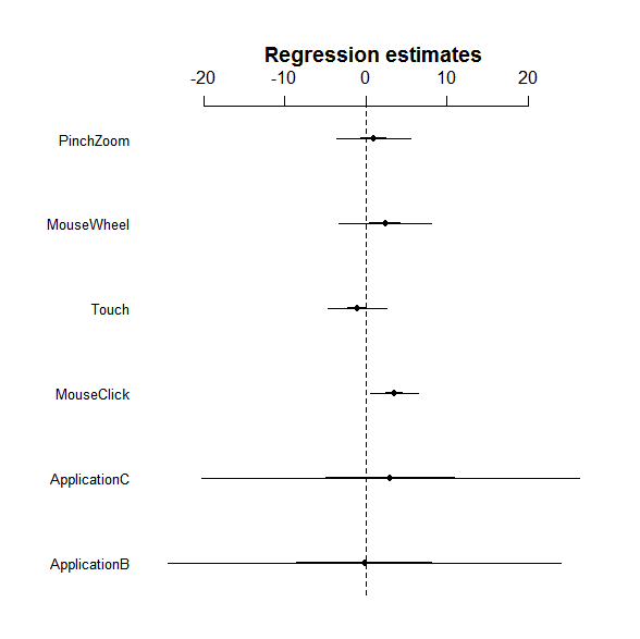
A thick and thin line represent the 1SD and 2SD ranges. So it looks like that MouseClick has a significant effect because its 2SD does not overlap the zero.

So far, so good. We successfully created a model and looks like we have something interesting there. But we are not quite sure about which fixed effects are significant yet.

If you have read the multiple linear regression page, you may think we can do an ANOVA test. Technically yes, we can do an ANOVA test. However, it is not quite straightforward to run it because of random effects. In this case, we cannot really be sure about whether the test statistic is F-distributed. There have been several attempts to address this and make an ANOVA test useful for multilevel regression, such as the Kenward-Roger correction. However, it is disputable if this correction is good enough so that we can assume the corrected test statistic is F-distributed. Thus, ANOVA with the Kenward-Roger correction has not been implemented yet in R (as of June 2011).

Instead, we use the Markov Chain Monte Carlo (MCMC) method to estimate the coefficient and highest probability density credible intervals (HPD credible intervals). Here, I will skip detailed discussions of what MCMC does and what HPD credible intervals mean. (I will do it sometime later at a separate page). For now, let's simply think that MCMC tries to re-estimate the coefficient for each factor based on the results we got with lmer() so that we can have better estimation.

We are going to use the languageR package to run MCMC. pvals.fnc() can take a bit of time for calculation.

The parameter nsim is the number of the simulation to run. Here, I set 10000, but you may need to tweak it to make sure that the estimation is converged.

MCMCmean is the re-estimated coefficient by MCMC. As you can see in this example, you may see relatively large differences between the estimation by REML and the one by MCMC. As far as I understand, the estimation by MCMC is more reliable than the one by REML. So we are going to use the results by MCMC.

As you can see in the results, only MouseClick has a significant positive effect on increasing performance time. So the results imply that reducing the number of mouse clicks may decrease the overall task completion time in the applications tested here. PinchZoom's effect (0.1278, 95% HPD CI:-5.1017,5.276) is smaller than MouseWheel (2.7309, 95% HPD CI:-3.8874, 9.867). Thus, encouraging users to do pinching gestures for zoom operations might contribute to decrease in the overall task completion time.

Unfortunately, there aren't many things to say from the results here, but I guess you have gotten the idea of how you interpret the results of multi-level linear models.

Lastly, let's make sure that we don't have multicollinearity problems. For lmer(), we cannot use the vif()function. Instead, we can use the function provided by Austin F. Frank (https://hlplab.wordpress.com/2011/02/24/diagnosing-collinearity-in-lme4/).

Copy the part of the vif.mer() function (or just copy all) in https://raw.github.com/aufrank/R-hacks/master/mer-utils.R, and paste them into your R console. And just use the vif.mer() function.

So, in this example, we are fine. If the value is higher than 5, you probably should remove that factor, and if it is higher than 2.5, you should consider removing it.

Another way to examine multicollinearlity is to look at the correlation of the two of the independent variables. I wrote a code to do this quickly.

Copy the code above, and paste it into your R console. Then, run the following code.

You will get the following graph.

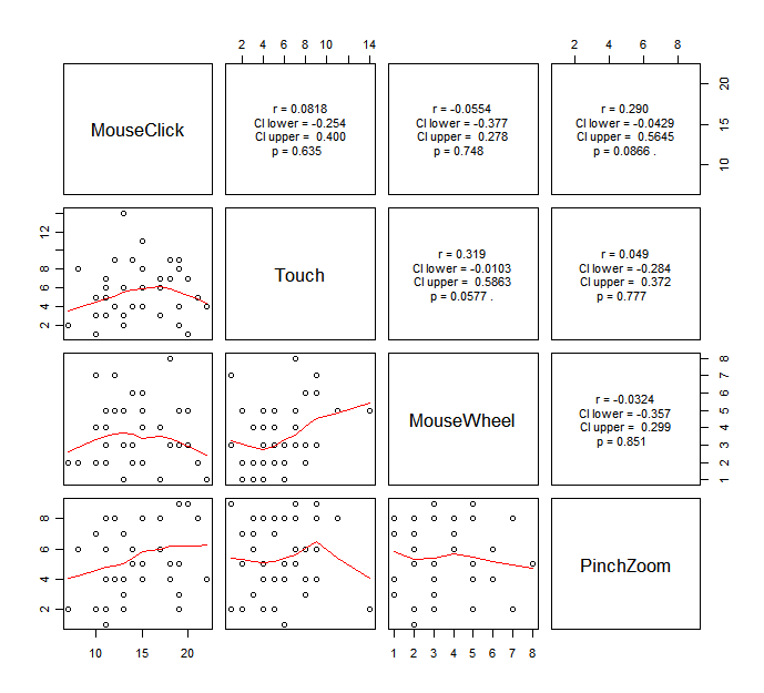
It is kinda hard to say which variable we should consider to remove from this, but I would say if you see any significant strong correlation, you probably should be careful about if it may cause multicollinearity.

Once you are done with your analysis, you will have to report the following things:

• Your model,
• How you chose the model (either you just defined, you used AIC, or you used CV),
• R-squared and adjusted R-squared (lmer() does not provide them, and I am looking into how to get them).
• How you tested the estimated coefficients (either you did MCMC or ran a F-test with the Kenward-Roger correction).
• Estimated value for each coefficient, and
• Significant effects with p value (if any).

For the last two items, you can say something like “MouseClick showed a significant effect (p<0.05). Its estimated coefficient with the MCMC method was 4.05 (95% HPD credible interval = [0.75, 7.63]).”

It is probably acceptable that you simply report the direction of each significant effect (positive or negative) if you do not really care about the actual value of the coefficient. But I think you should report at least whether each significant effect contributes to the dependent variable in a positive or negative way.