Table of Contents
Post-hoc Tests
Introduction
If you find any significant main effect or interaction with an ANOVA test, congrats, you have at least one significant difference in your data. However, an ANOVA test doesn't tell you where you have the differences. Thus, you need to do one more test–a post-hoc test–to find where they exist.
Comparisons for main effects
As we have seen in the Anova page, there are two kinds of effects you may have: main effects, and interactions (if your model is two-way or more). The comparison for the main effect is fairly straightforward, but there are four kinds of comparisons you can make, so you have to decide which one you want to do.
Before talking about the differences of the comparisons, you need to know one important thing. Some of the post-hoc comparisons may not be appropriate for repeated-measure ANOVA. I am not 100% sure about this point, but it seems that some of the methods do not consider the within-subject design. So, my current suggestion is that if the factor you are comparing in a post-hoc test is a within-subject factor, it might be safer to use a t test with the Bonferroni's or Sidak's correction.
OK., back to the discussion about the types of comparisons. For the discussion, let's say you have three groups: A, B, and C.
- [Case 1] Compare every possible combination of your groups: In this case, you compare everything. You will compare A and B, B and C, and C and A. But you also compare A and B+C (the mean of B and C), B and C+A, C and A+B.
- [Case 2] Compare every group: In this case, you will compare A and B, B and C, and C and A. But you do not compare A and B+C, B and C+A, C and A+B.
- [Case 3] Compare every group against the control: In this case, you will compare the groups only against the control condition. If your control condition is A, you will compare A and B, and A and C.
- [Case 4] Compare the data against the within-subject factor: In this case, you will make a comparison against the within-subject factor. In other words, if you have done repeated-measure ANOVA, this is the way to do a post-hoc test. The methods for this case can be used for tests against between-subject factors.
The strict definition of a post-hoc test means a test which does not require any plan for testing. In the four examples above, only Case 1 satisfies the strict definition of a post-hoc test because the others cases require some sort of planning on which groups to compare or not to compare. However, the term of a post-hoc test is often used for meaning Case 2 and Case 3. Case 4 is usually called a planned comparison test, but again it is often referred as a post-hoc test as well. In this wiki, I use a post-hoc test to mean all of these four tests.
The key point here is you need to figure out which case you want to do for the comparisons after ANOVA. Make sure what comparisons you are interested in before doing any test.
Comparisons for interactions
If you find a significant interaction, things are a little more complicated. This means that the effect of one factor depends on the conditions controlled by the other factors. So, what you need to do is to make comparisons against one factor with fixing the other factors. Let's say you have two Devices (Pen and Touch) and three Techniques (A, B, and C) as we have seen in the two-way ANOVA example. If you have found the interaction, what you need to look at is:
- The effect of Technique under Device = Pen;
- The effect of Technique under Device = Touch;
- The effect of Device under Technique = A;
- The effect of Device under Technique = B; and
- The effect of Device under Technique = C.
The effects we look at here are called simple main effects. Although you could report all the simple main effects you have, it might become lengthy. Rather, providing a graph like above is easier to understand what kinds of trends your data have. Your graph will look like one of the following graphs depending of the existence of main effects and interactions.
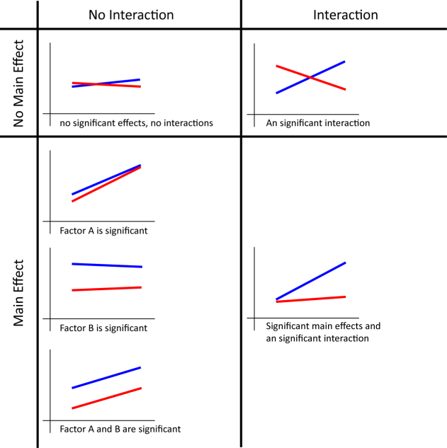
It is also said that you shouldn't report the main effects (not simple main effects) when you have a significant interaction. This is because significant differences are caused by some combination of the factors, and not necessarily caused by a single factor. However, I think that it is still good to report any significant main effects even if you have a significant interaction because it tells us what the data look like. Again, providing a graph is very helpful for your readers to understand your data.
The sad news is that it is not as easy in R to do post-hoc test as in SPSS. You often have to do a lot of things manually or some methods are not really supported in R. So, particularly if you are doing two-way ANOVA and you have an access to SPSS, it may be better to use SPSS.
Main effect: Comparing every possible combination of your groups (Scheffe's test)
Scheffe's test allows you to do a comparison on every possible combination of the group you are caring about. Unfortunately, there is no automatic way to do Scheffe's test in R. You have to do it manually. The following procedure is based on Colleen Moore & Mike Amato's material.
We use the same example for one-way ANOVA.
We have a significant effect of Group. So, we need to look into that effect more deeply. First, you have to define the combination of the groups for your comparison.
The each element of coeff intuitively means the weight for the later calculation. The positive values and negative values represent data to compare. In this case, the first element is 1, and the second element is -1. And the first, second, and third elements will represent Group A, B, and C, respectively. So, this coeff means we are going to compare Group A and Group B. The third element is 0, which means Group C will be ignored.
Another key point is the sum of the elements must be 0. Here are some other examples.
- If you have three groups (A, B, C), and you want to compare Group B and C, coeff = c(0, 1, -1).
- If you have three groups (A, B, C), and you want to compare Group A and the mean of Group B and C, coeff = c(2, -1, -1).
- If you have five groups (A, B, C, D, E), and you want to compare the mean of Group A and B, and the mean of Group C, D and E, coeff = c(2/3, 2/3, 2/3, -1, -1).
Let's come back to the example. Now we need to calculate the number of the samples and the mean for each group.
We then calculate some statistical values.
mspsi should be 7.5625 if you have followed the example correctly. Now we are going to calculate the F value. For this, we need to know the value for the mean square for the errors (or residuals). According to the result of the anova test, it is 0.9405 (Did you find it? Go back to the very first of this example and see the result of summary(aov)). We also need to know the degree of freedom of the factor we are caring about (in this example, Group), which is 2.
Finally, we can calculate the p value for this comparison (comparison between Group A and Group B). For the degrees of freedom, we can use the same ones for the anova test, which is 2 for the first DOF, 21 for the second DOF (Find them in the result of the anova test).
Thus, the difference between Group A and B is significant because p < 0.05.
So, if you really want to do all possible comparisons, you probably want to write some codes so that you can do a batch operation. I think it should be straightforward, but be careful about the design of the comparison (i.e., coeff).
I am not 100% sure, but Scheffe's test may not be appropriate for repeated-measure ANOVA. For repeated-measure ANOVA, you can do a pairwise comparison with the Bonferroni's or Sidak's correction.
Main effect: Comparing every group (Tukey's test)
This is probably the most common case in HCI research. You want to compare the two of the groups, but you are not interested in any combination of more than one group. One of the common methods for this case is Tukey's method. The way to do a Tukey's test in R depends on how you have done ANOVA.
First, let's take a look at how to do a Tukey's test with the aov() function. We use the same example of one-way ANOVA.
Now, we do a Tukey's test.
So, we have significant differences between A and B, and A and C.
If you use the Anova() function, the way to do a Tukey's test is a little different. Here, we use the same example of two-way ANOVA, but the values for Time were slightly changed (to make the interaction effect disappear).
With the anova test, you will find the main effects. So, you need to run a Tukey's test. You have to do the following thing to do a Tukey's test with the model created by lm(). You need to include multcomp package beforehand.
Then, you get the results.
So, we have significant differences between any of the two groups in both Device and Technique.
It seems both ways to do a Tukey's test can accommodate mildly unbalanced data (the number of the samples are different cross the groups, but not that different). The Tukey's test which can handle mildly unbalanced data is also called Tukey-Kramer's test. If you have largely unbalanced data, you can't do a Tukey's test nor even ANOVA, and instead you should do a non-parametric test.
Another thing you should need to know is that Tukey may not be appropriate as a post-hoc test for repeated-measure ANOVA. This is because Tukey assumes the independency of the data across the groups. You can actually run a Tukey's test even for repeated-measure ANOVA with the second method (you need to use lme() in nlme package to build a model instead of lm()). As far as I can tell, it seems ok to use a Tukey's test for repeated-measure data, but I am not 100% sure yet.
With some statistical software, you can also run a Tukey's test for an interaction term. Unfortunately, it seems that it is not possible to do so in R (as of July 2011). I think this makes sense because you can simply look at simple main effects if you have a significant interaction term. But if you know a way to run a Tukey's test for an interaction term, please let me know.
Main effect: Comparing every group against the control (Dunnett's test)
In this case, you have one group which can be called “the reference group”, and you want to compare the groups only against this reference group. One common test is a Dunnett's test, and fortunately the way to do a Dunnett's test is as easy as a Tukey's test.
Let's use an example of the one-way ANOVA test.
Now, you are going to do a Dunnett's test. You need to include multcomp package.
As you can see in the result, the Dunnett's test only did comparisons between Technique A and B, and between Technique A and C. In this method, the first group in the factor you are caring about is used as the reference case (in this example, Technique A). So, you need to design the data so that the data for the reference case are associated with the first group in the factor.
You may have also noticed that the p values become smaller than those in the results of a Tukey's test.
| Tukey | Dunnett | |
|---|---|---|
| A - B | 0.0257122 | 0.018472 |
| A - C | 0.0002167 | 0.000149 |
Generally, a Dunnett's test is more sensitive (has more powers to find a significant difference) than a Tukey's test. At a cost of this power, you must assume the reference case for the comparisons.
You can also use the model generated by aov() in the lm() function. Here is another example of a Dunnett's test for two-way ANOVA.
Now, you get the result.
Main effect: Comparing data against the within-subject factor (Bonferroni correction, Holm method)
Another case you would commonly have is that you have within-subject factors. Unfortunately, in this case, the methods explained above may not be appropriate because they do not take the relationship between the groups into account. Instead, you can do a paired t test with some corrections to avoid some troubles caused by doing multiple t tests. The major corrections are Bonferroni correction and Holm method. Fortunately, you can do both quite easily in R. Let's take a look at the example of one-way repeated-measure ANOVA.
Doing multiple t tests with Bonferroni correction is as follows.
If you want to use Holm method, you just need to change the value of p.adj (or remove the argument of p.adj completely. R uses Holm method by default).
Other kinds of corrections are also available (type ?p.adjust.methods in the R console). But I think these two are usually good enough. It is considered that you should avoid using Bonferroni correction when you have more than 4 groups to compare. This is because Bonferroni correction becomes too strict for those cases.
You can also use the methods above for between-subject factors instead of using other methods (like Tukey's test). In this case, you just need to do something like:
So, which one to use?
There are several other things which may help you choose a particular method in addition to the properties explained above.
- A Dunnet's test has a stronger power (more likely to find a significant difference) than other methods. (But you need to assume the reference case).
- A Tukey's test (or Tukey-Kramer's test) is more strict or conservative (less likely to find a significant difference) than the pairwise comparison with the Bonferroni correction when the number of the groups to compare is small. But when the number of the groups to compare is large, a Tukey's test becomes less strict than the pairwise comparison with the Bonferroni correction.
- The pairwise comparison with the Bonferroni correction often becomes too strict when the number of the groups to compare is large. Generally, when the number of the groups is more than six, we want to avoid using this.
- A Scheffe's test tends to be strict because it compares all possible combination.
In HCI research, the most common method I have seen is either a Tukey's test or pairwise comparison with the Bonferroni correction. So, if you don't have any particular comparison in mind, these two would be the first thing you may want to try.
Interaction
If you have any significant interaction, you need to look at the data more carefully because more than 0ne factor contribute to significant differences. There are two ways to look into the data: simple main effects and interaction contrasts.
Simple main effect
The idea of the simple main effect is very intuitive. If you have n factors, you pick up one of them, fix it, and do a test for the n-1 factors. In our two-way ANOVA example, there are five tests for looking at simple main effects:
- A comparison against Technique for the data with Device = Pen;
- A comparison against Technique for the data with Device = Touch;
- A comparison against Device for the data with Technique = A;
- A comparison against Device for the data with Technique = B; and
- A comparison against Device for the data with Technique = C.
Let's do it with the example of two-way ANOVA.
This ANOVA test shows you have a significant interaction, so now we are going to look at the simple main effects. First, we are going to look at the difference caused by Technique for the Pen condition. For this, we pick up data only for the Pen condition.
We can then simply run a one-way ANOVA test against Technique.
So, we have a significant simple effect here. We can do tests for other simple main effects in a similar way.
If you only have two groups to compare, you can just do a t test as you can see above. In this example, you will find significant simple effects in all the five tests. But if the main effects are so powerful, we cannot find clear interactions of the factors with tests for simple main effects. In such cases, we need to switch to doing tests for interaction contrasts.
Interaction Contrast
Interaction contrasts basically mean you compare every combination of the two groups. So it seems kind of similar to Scheffe's test. I haven't figured out how to do interaction contrasts in R. I will add it when I figure out.
Do I really need to run ANOVA?
Some of you may have noticed that some post-hoc test methods explained here do not use any result gained from aov() or Anova() function. For example. post-hoc tests with Bonferroni or Holm correction do not use the results of the ANOVA test.
In theory, if you use post-hoc methods which do not require the result of the ANOVA test, you don't need to run ANOVA, and can directly run post-hoc methods. However, running ANOVA and then running post-hoc tests is kind of a de-facto standard, and most of the readers expect the results of ANOVA (and the results of post-hoc tests in the case you find any statistical difference through the ANOVA test). Thus, in order to avoid the confusion that the reader might have, it is probably better to run ANOVA regardless of whether it is theoretically needed.
How to report
In the report, you need to describe which post-hoc test you used and where you found the significant differences. Let's say you are using a Tukey's test and have the results like this.
Then, you should report as follows:
A Tukey's pairwise comparison revealed the significant differences between A and B (p < 0.05), and between A and C (p < 0.01).
Of course, you need to report the results of your ANOVA test before this.